- 参考《30分钟学会ggplot2》肖凯,基本概念
1. 用mpg生成散点图
library("ggplot2") #载入ggplot2;
str(mpg) #查看mpg数据集的变量类型
## Classes 'tbl_df', 'tbl' and 'data.frame': 234 obs. of 11 variables:
## $ manufacturer: chr "audi" "audi" "audi" "audi" ...
## $ model : chr "a4" "a4" "a4" "a4" ...
## $ displ : num 1.8 1.8 2 2 2.8 2.8 3.1 1.8 1.8 2 ...
## $ year : int 1999 1999 2008 2008 1999 1999 2008 1999 1999 2008 ...
## $ cyl : int 4 4 4 4 6 6 6 4 4 4 ...
## $ trans : chr "auto(l5)" "manual(m5)" "manual(m6)" "auto(av)" ...
## $ drv : chr "f" "f" "f" "f" ...
## $ cty : int 18 21 20 21 16 18 18 18 16 20 ...
## $ hwy : int 29 29 31 30 26 26 27 26 25 28 ...
## $ fl : chr "p" "p" "p" "p" ...
## $ class : chr "compact" "compact" "compact" "compact" ...p<-ggplot(mpg,mapping=aes(x=cty,y=hwy)) #以mpg为数据集,将变量cty(在城市中每加仑油跑的距离),hwy(高速公路)mapping(映射)到x.y(aesthetics)轴上。
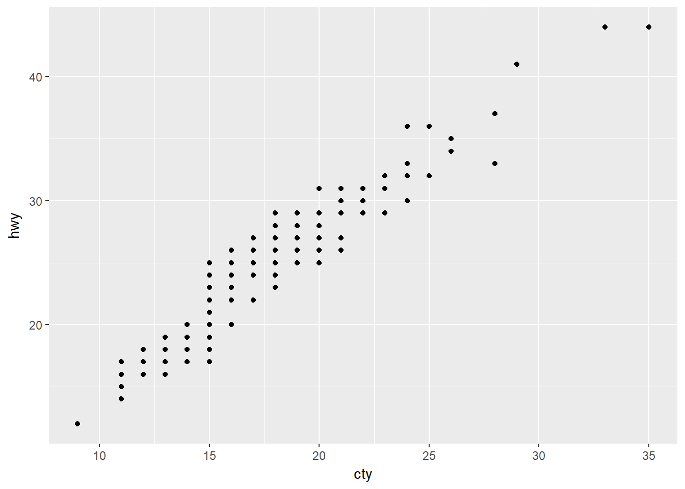
p+geom_point() #在图上加上几何对象:点(geometric piont)
p ;p+geom_point()#展示
summary(p);summary(p+geom_point()) #查看对象的摘要描述## data: manufacturer, model, displ, year, cyl, trans, drv, cty, hwy,
## fl, class [234x11]
## mapping: x = cty, y = hwy
## faceting: <ggproto object: Class FacetNull, Facet>
## compute_layout: function
## draw_back: function
## draw_front: function
## draw_labels: function
## draw_panels: function
## finish_data: function
## init_scales: function
## map: function
## map_data: function
## params: list
## render_back: function
## render_front: function
## render_panels: function
## setup_data: function
## setup_params: function
## shrink: TRUE
## train: function
## train_positions: function
## train_scales: function
## vars: function
## super: <ggproto object: Class FacetNull, Facet>## data: manufacturer, model, displ, year, cyl, trans, drv, cty, hwy,
## fl, class [234x11]
## mapping: x = cty, y = hwy
## faceting: <ggproto object: Class FacetNull, Facet>
## compute_layout: function
## draw_back: function
## draw_front: function
## draw_labels: function
## draw_panels: function
## finish_data: function
## init_scales: function
## map: function
## map_data: function
## params: list
## render_back: function
## render_front: function
## render_panels: function
## setup_data: function
## setup_params: function
## shrink: TRUE
## train: function
## train_positions: function
## train_scales: function
## vars: function
## super: <ggproto object: Class FacetNull, Facet>
## -----------------------------------
## geom_point: na.rm = FALSE
## stat_identity: na.rm = FALSE
## position_identity2.将年份映射到颜色属性上
p<-ggplot(mpg,mapping = aes(x = cty,y = hwy,colour = factor(year)))
p+geom_point()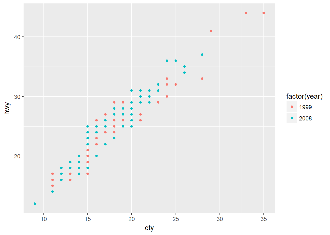 #### 3.添加平滑曲线
p+geom_point()+stat_smooth()## `geom_smooth()` using method = 'loess'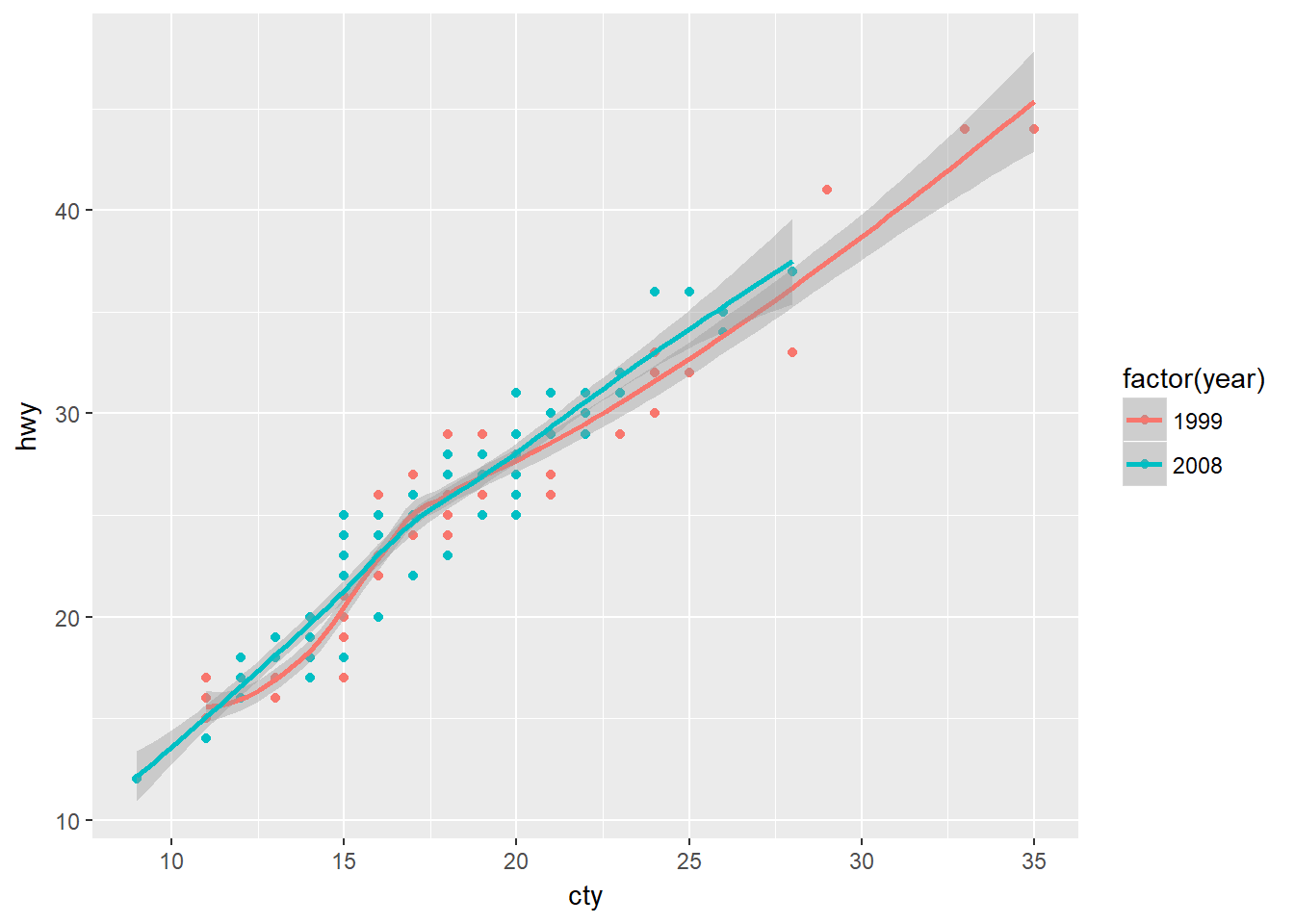
rm(p) #清楚变量p,将年份只映射到点的颜色属性上P pP
p <- ggplot(mpg, aes(x=cty,y=hwy))
p + geom_point(aes(colour=factor(year)))+stat_smooth()
## `geom_smooth()` using method = 'loess'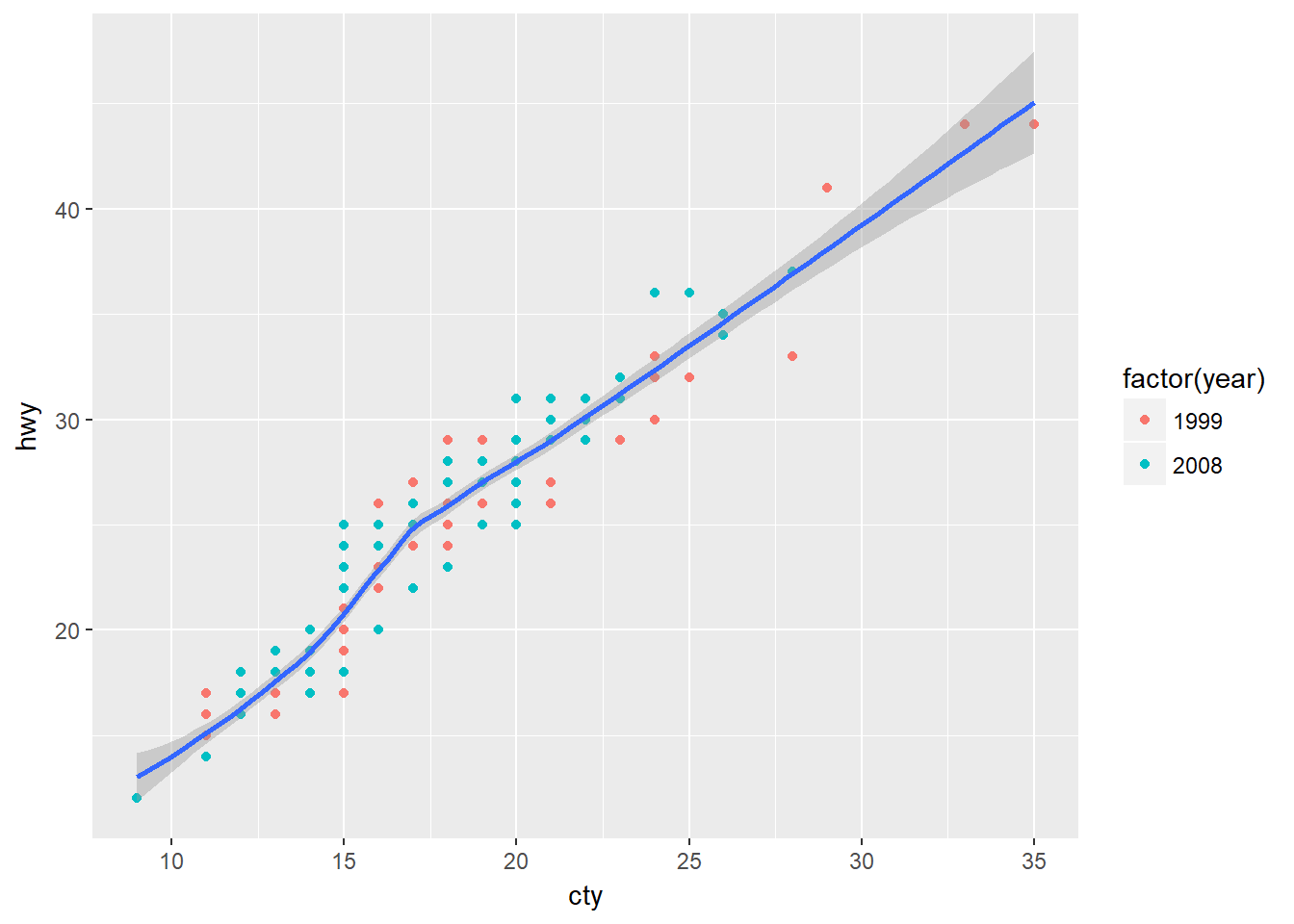 #### 4.换种思路绘一遍
d <- ggplot() +
geom_point(data=mpg, aes(x=cty, y=hwy, colour=factor(year)))+
stat_smooth(data=mpg, aes(x=cty, y=hwy))
#必须明确data eg no:d<-ggplot()+geom_point(mpg,aes(x=cty,y=hwy,colour=factor(year)))+stat_smooth(mpg,aes(x=cty,y=hwy))
# 原因:ggplot与geom_各自的data与mapping的位置不一致,eg yes:d<-ggplot()+geom_point(aes(x=cty,y=hwy,colour=factor(year)),mpg)+stat_smooth(aes(x=cty,y=hwy),mpg)
print(d)#此时除了底层画布外,有两个图层,分别定义了geom和 stat。
## `geom_smooth()` using method = 'loess' #### 5.用标度(scale)来修改颜色取值
scale_color_manual说明:This allows you to specify you own set of mappings from levels in the data to aesthetic values.
d+scale_color_manual(values = c("yellow","red"))## `geom_smooth()` using method = 'loess'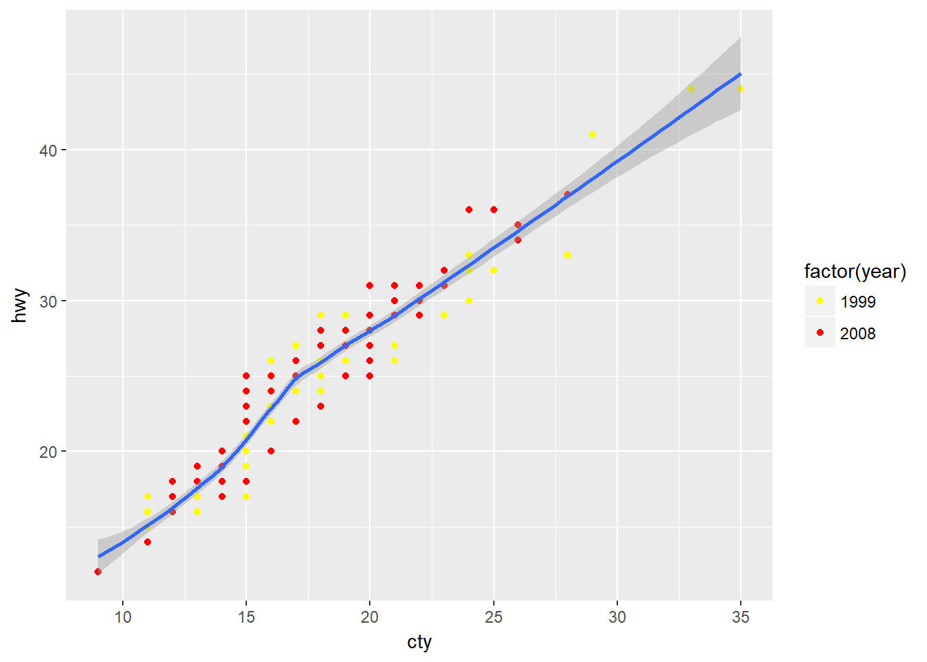 #### 6.将排量映射到散点的大小上
d <- ggplot() +
geom_point(data=mpg, aes(x=cty, y=hwy, colour=factor(year),size=displ),alpha=0.5,position = "jitter")+
stat_smooth(data=mpg, aes(x=cty, y=hwy))
d+scale_color_manual(values = c("yellow","red"))+coord_cartesian(xlim = c(15, 25),ylim=c(15,40)) #用坐标控制图形显示的范围
## `geom_smooth()` using method = 'loess'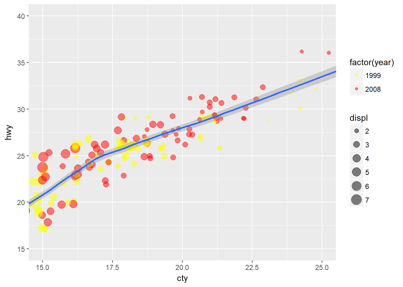 #### 7.用facet(分面)显示不同年份的数据
d <- ggplot() +
geom_point(data=mpg, aes(x=cty, y=hwy, colour=factor(year),size=displ),alpha=0.5,position = "jitter")+
stat_smooth(data=mpg, aes(x=cty, y=hwy))
d+scale_color_manual(values = c("yellow","red"))+coord_cartesian(xlim = c(15, 25),ylim=c(15,40))+facet_wrap(~year,nrow=2)
## `geom_smooth()` using method = 'loess'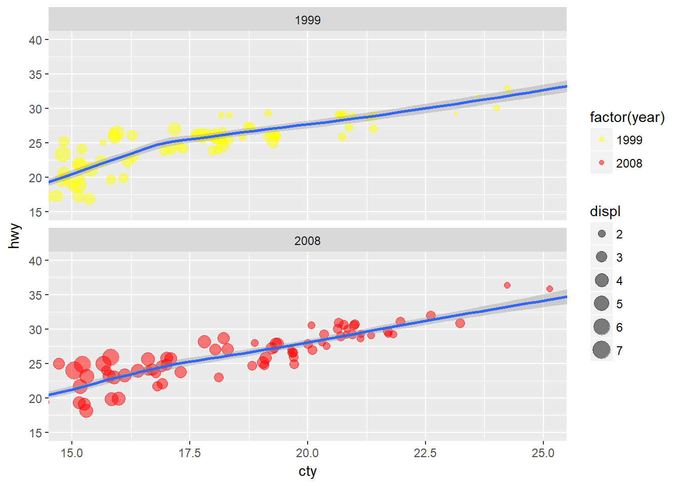 #### 6.增加图名幵精细修改图例
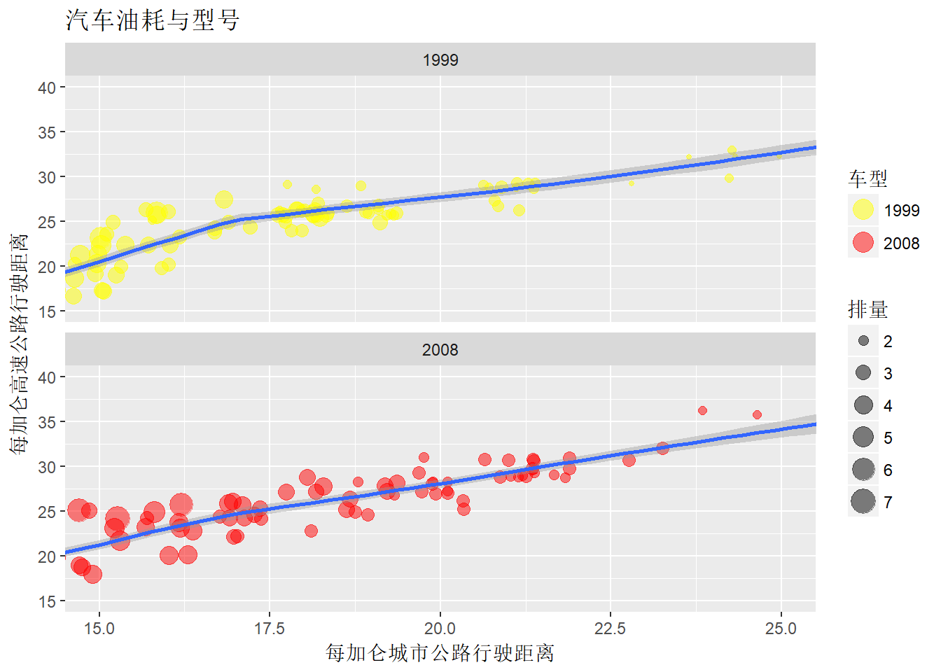
d <- ggplot() +
geom_point(data=mpg, aes(x=cty, y=hwy, colour=factor(year),size=displ),alpha=0.5,position = "jitter")+
stat_smooth(data=mpg, aes(x=cty, y=hwy))
d+scale_color_manual(values = c("yellow","red"))+coord_cartesian(xlim = c(15, 25),ylim=c(15,40))+facet_wrap(~year,nrow=2)+
labs(y='每加仑高速公路行驶距离',x='每加仑城市公路行驶距离')+guides(size=guide_legend(title='排量'),colour = guide_legend(title='车型',override.aes=list(size=5)))+ggtitle('汽车油耗与型号')#不知道怎么居中
## `geom_smooth()` using method = 'loess'