- demo演示
R可以构建复杂的立体图形 结合ggplot2绘制的图形更加精美
\[\int_0^\infty e^{-x^2} dx=\frac{\sqrt{\pi}}{2}\]
demo(persp)##
##
## demo(persp)
## ---- ~~~~~
##
## > ### Demos for persp() plots -- things not in example(persp)
## > ### -------------------------
## >
## > require(datasets)
##
## > require(grDevices); require(graphics)
##
## > ## (1) The Obligatory Mathematical surface.
## > ## Rotated sinc function.
## >
## > x <- seq(-10, 10, length.out = 50)
##
## > y <- x
##
## > rotsinc <- function(x,y)
## + {
## + sinc <- function(x) { y <- sin(x)/x ; y[is.na(y)] <- 1; y }
## + 10 * sinc( sqrt(x^2+y^2) )
## + }
##
## > sinc.exp <- expression(z == Sinc(sqrt(x^2 + y^2)))
##
## > z <- outer(x, y, rotsinc)
##
## > oldpar <- par(bg = "white")
##
## > persp(x, y, z, theta = 30, phi = 30, expand = 0.5, col = "lightblue")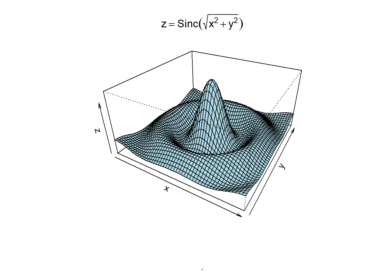
##
## > title(sub=".")## work around persp+plotmath bug
##
## > title(main = sinc.exp)
##
## > persp(x, y, z, theta = 30, phi = 30, expand = 0.5, col = "lightblue",
## +       ltheta = 120, shade = 0.75, ticktype = "detailed",
## +       xlab = "X", ylab = "Y", zlab = "Z")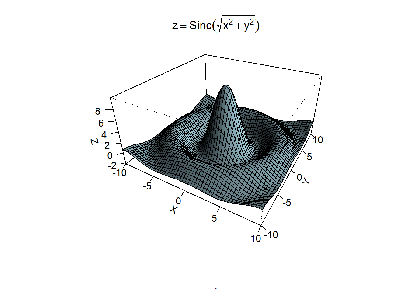
##
## > title(sub=".")## work around persp+plotmath bug
##
## > title(main = sinc.exp)
##
## > ## (2) Visualizing a simple DEM model
## >
## > z <- 2 * volcano        # Exaggerate the relief
##
## > x <- 10 * (1:nrow(z))   # 10 meter spacing (S to N)
##
## > y <- 10 * (1:ncol(z))   # 10 meter spacing (E to W)
##
## > persp(x, y, z, theta = 120, phi = 15, scale = FALSE, axes = FALSE)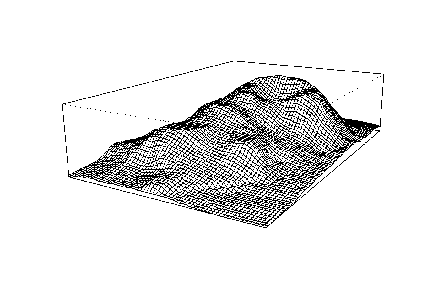
##
## > ## (3) Now something more complex
## > ##     We border the surface, to make it more "slice like"
## > ##     and color the top and sides of the surface differently.
## >
## > z0 <- min(z) - 20
##
## > z <- rbind(z0, cbind(z0, z, z0), z0)
##
## > x <- c(min(x) - 1e-10, x, max(x) + 1e-10)
##
## > y <- c(min(y) - 1e-10, y, max(y) + 1e-10)
##
## > fill <- matrix("green3", nrow = nrow(z)-1, ncol = ncol(z)-1)
##
## > fill[ , i2 <- c(1,ncol(fill))] <- "gray"
##
## > fill[i1 <- c(1,nrow(fill)) , ] <- "gray"
##
## > par(bg = "lightblue")
##
## > persp(x, y, z, theta = 120, phi = 15, col = fill, scale = FALSE, axes = FALSE)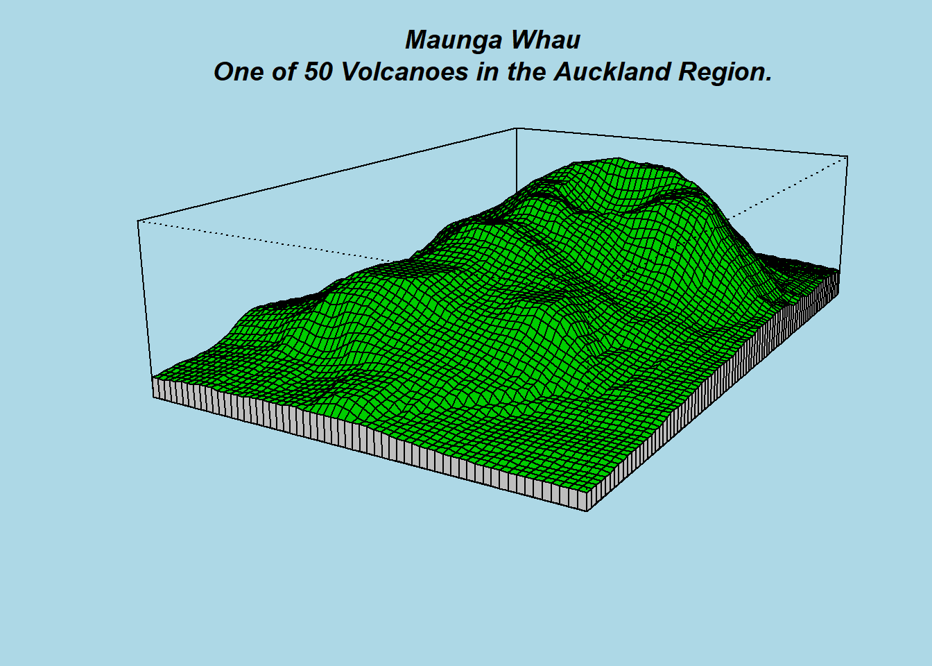
##
## > title(main = "Maunga Whau\nOne of 50 Volcanoes in the Auckland Region.",
## +       font.main = 4)
##
## > par(bg = "slategray")
##
## > persp(x, y, z, theta = 135, phi = 30, col = fill, scale = FALSE,
## +       ltheta = -120, lphi = 15, shade = 0.65, axes = FALSE)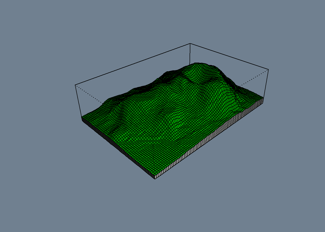
##
## > ## Don't draw the grid lines :  border = NA
## > persp(x, y, z, theta = 135, phi = 30, col = "green3", scale = FALSE,
## +       ltheta = -120, shade = 0.75, border = NA, box = FALSE)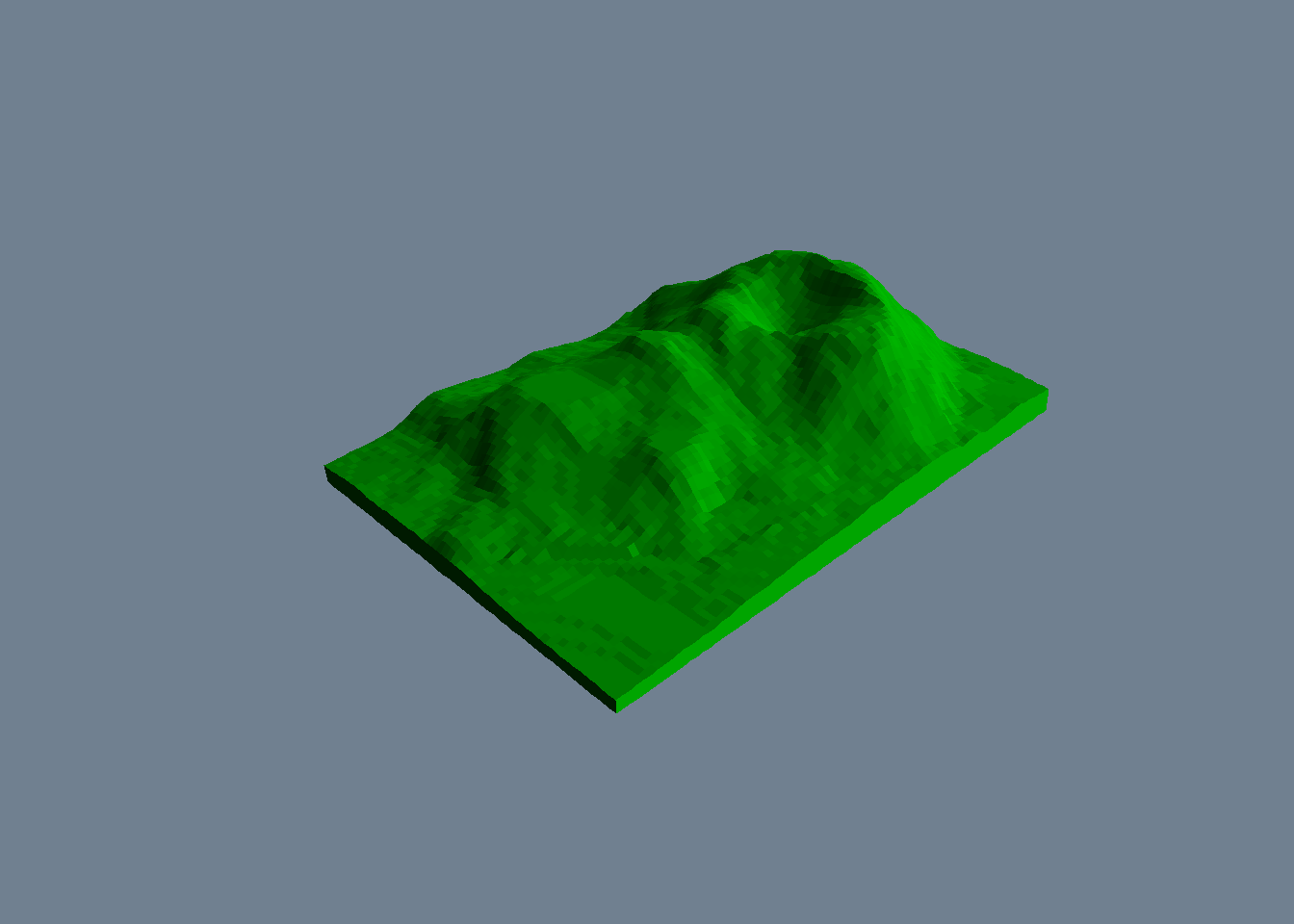
##
## > ## `color gradient in the soil' :
## > fcol <- fill ; fcol[] <- terrain.colors(nrow(fcol))
##
## > persp(x, y, z, theta = 135, phi = 30, col = fcol, scale = FALSE,
## +       ltheta = -120, shade = 0.3, border = NA, box = FALSE)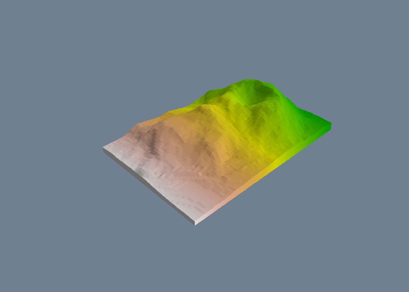
##
## > ## `image like' colors on top :
## > fcol <- fill
##
## > zi <- volcano[ -1,-1] + volcano[ -1,-61] +
## +            volcano[-87,-1] + volcano[-87,-61]  ## / 4
##
## > fcol[-i1,-i2] <-
## +     terrain.colors(20)[cut(zi,
## +                            stats::quantile(zi, seq(0,1, length.out = 21)),
## +                            include.lowest = TRUE)]
##
## > persp(x, y, 2*z, theta = 110, phi = 40, col = fcol, scale = FALSE,
## +       ltheta = -120, shade = 0.4, border = NA, box = FALSE)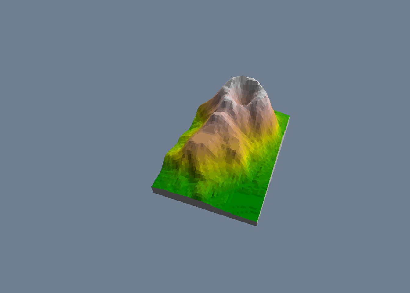
##
## > ## reset par():
## > par(oldpar)